This example illustrates the effects of time-varying sources on estimation. The example also shows how to set time-varying sources to be constant during estimation to improve estimation results.
Open the Simulink® model.
sys = 'scdspeed_ctrlloop';
open_system(sys)
Linearize the model.
Set the Engine Model block to normal
mode for accurate linearization.
set_param('scdspeed_ctrlloop/Engine Model','SimulationMode','Normal')
Open the Model Linearizer for the model.
In the Simulink model window, in the Apps gallery, click Model Linearizer.
Click ![]() Bode to linearize the model
and generate a Bode plot of the result.
Bode to linearize the model
and generate a Bode plot of the result.
The linearized model, linsys1, appears in
the Linear Analysis Workspace.
Create an input sinestream signal for the estimation.
Open the Create sinestream input dialog box.
In the Estimation tab, in the Input Signal drop-down list, select Sinestream.
Open the Add frequencies dialog box.
Click ![]() .
.
Specify the input sinestream frequency range and number of frequency points.
Enter 10 in the From box.
Enter 100 in the To box.
Enter 10 in the box for the number of frequency
points.
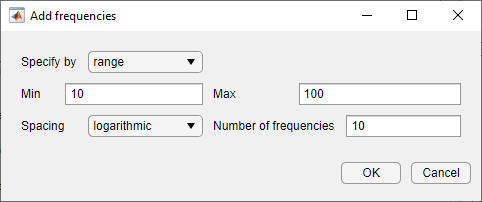
Click OK.
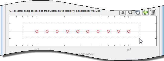
The added points are visible in the frequency content viewer of the Create sinestream input dialog box.
In the frequency content viewer of the Create sinestream input dialog box, select all the frequency points.
Specify input sinestream parameters.
Change the Number of periods and Settling periods to ensure that the model reaches steady-state for each frequency point in the input sinestream.
Enter 30 in the Number of periods box.
Enter 25 in the Settling periods box.
Create the input sinestream.
Click OK. The new input signal, in_sine1,
appears in the Linear Analysis Workspace.
Set the Diagnostic Viewer to open when estimation is performed.
Select the Launch Diagnostic Viewer check box.
Estimate the frequency response for the model.
Click ![]() Bode Plot 1 to estimate
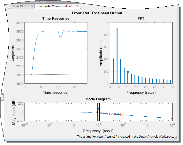
the frequency response. The Diagnostic Viewer appears in the plot
plane and the estimated system
Bode Plot 1 to estimate
the frequency response. The Diagnostic Viewer appears in the plot
plane and the estimated system estsys1, appears
in the Linear Analysis Workspace.
Compare the estimated model and the linearized model.
Click on the Diagnostic Viewer - estsys1 tab in the plot area of the Model Linearizer.
Click and drag linsys1 onto the
Diagnostic Viewer to add linsys1 to the Bode
Diagram.
Click the Diagnostic Viewer tab.
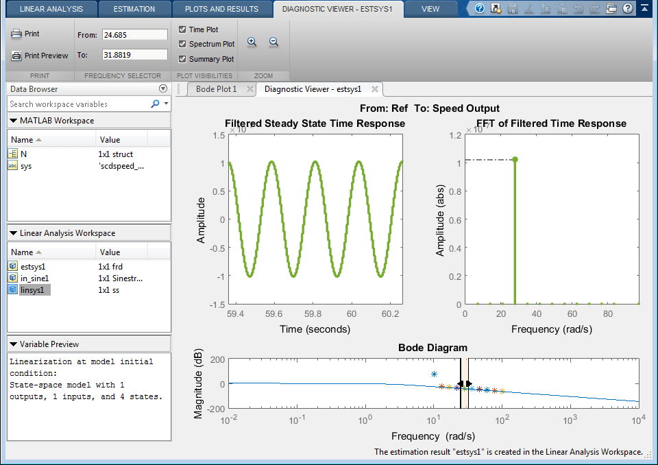
Configure the Diagnostic Viewer to show only the frequency point where the estimation and linearization results do not match.
In the Frequency Selector section, enter 9 in
the From box and 11 in the To box
to set the frequency range that is analyzed in the Diagnostic Viewer.
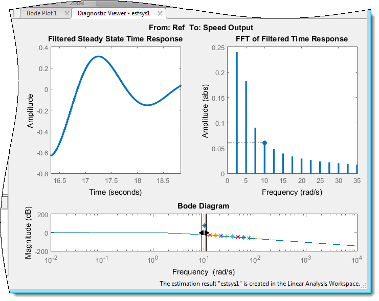
The Filtered Steady State Time Response plot shows a signal that is not sinusoidal.
View the unfiltered time response.
Right-click the Filtered Steady State Time Response plot and clear the Show filtered steady state output only option.
The step input and external disturbances drive the model away from the operating point that the linearized model uses. This prevents the response from reaching steady-state. To correct this problem, find and disable the time-varying source blocks that interfere with the estimation. Then estimate the frequency response of the model again.
Find and disable the time-varying sources within the model.
Open the Options for frequency response estimation dialog box.
On the Estimation tab, in the Options section, click More Options.
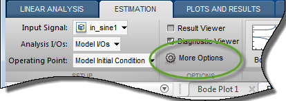
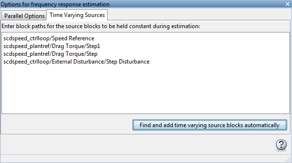
In the Time Varying Sources tab, click Find and add time varying source blocks automatically.
This action populates the time varying sources list with the block paths of the time varying sources in the model. These sources will be held constant during estimation.
Estimate the frequency response for the model.
Click ![]() Bode Plot 1 to estimate
the frequency response. The estimated system
Bode Plot 1 to estimate
the frequency response. The estimated system estsys2,
appears in the Linear Analysis Workspace.
Compare the newly estimated model and the linearized model.
Click on the Diagnostic Viewer - estsys2 tab in the plot area of the Model Linearizer.
Click and drag linsys1 onto the Diagnostic
Viewer.
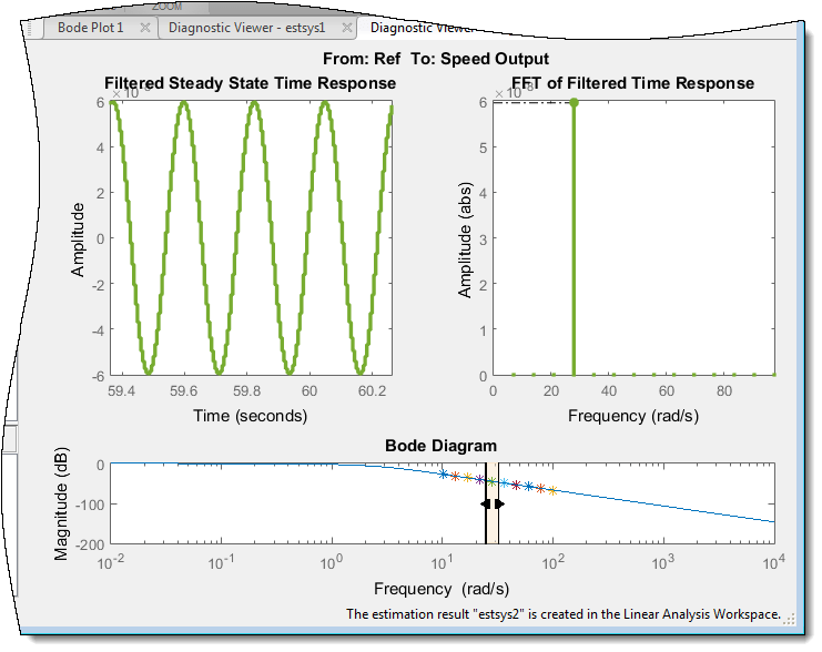
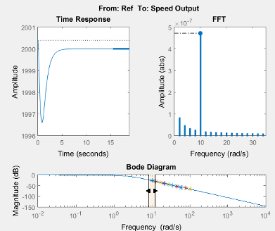
The frequency response obtained by holding the time-varying sources constant matches the exact linearization results.
Compare the linear model obtained using exact linearization techniques with the estimated frequency response:
% Open the model
mdl = 'scdspeed_ctrlloop';
open_system(mdl)
io = getlinio(mdl);

% Set the model reference to normal mode for accurate linearization
set_param('scdspeed_ctrlloop/Engine Model','SimulationMode','Normal')

% Linearize the model
sys = linearize(mdl,io);

% Estimate the frequency response between 10 and 100 rad/s
in = frest.Sinestream('Frequency',logspace(1,2,10),'NumPeriods',30,'SettlingPeriods',25);
[sysest,simout] = frestimate(mdl,io,in);

% Compare the results
frest.simView(simout,in,sysest,sys)
The linearization results do not match the estimated frequency response for the first two frequencies. To view the unfiltered time response, right-click the time response plot, and clear Show filtered steady state output only.
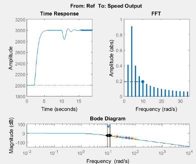
The step input and external disturbances drive the model away from the operating point, preventing the response from reaching steady-state. To correct this problem, find and disable these time-varying source blocks that interfere with the estimation.
Identify the time-varying source blocks using frest.findSources.
srcblks = frest.findSources(mdl,io);
Create a frestimate options set to disable
the blocks.
opts = frestimateOptions;
opts.BlocksToHoldConstant = srcblks;
Repeat the frequency response estimation using the optional
input argument opts.
[sysest2,simout2] = frestimate(mdl,io,in,opts);
frest.simView(simout2,in,sysest2,sys)
Now the resulting frequency response matches the exact linearization results. To view the unfiltered time response, right-click the time response plot, and clear Show filtered steady state output only.
Some time-varying source blocks might not be found by the algorithm. If the internal
signal path of a block does not contain a block with no input port, that block is not
reported by the frest.findSources function or in the app.
To bring the model to steady state, replace the source block with a Constant block, or a different source block.
