Initialize Steady-State Operating Point Search Using Simulation Snapshot

If you know the approximate time when the model reaches the neighborhood of a steady-state operating point, you can use simulation to get state values to use as the initial conditions for numerical optimization.

Initialize Operating Point Search Using Steady State Manager

You can initialize operating point searches with a simulation snapshot when computing operating points using the Steady State Manager.

Open the Simulink^® model.
```
sys = 'watertank';
open_system(sys)
```
To open the Steady State Manager, in the Simulink model window, in the Apps gallery, click Steady State Manager.
In the Steady State Manager, on the Steady State tab, click Snapshots.
In the Create Snapshot Operating Point dialog box, enter 10 in the Simulation snapshot times field to extract the operating point at this simulation time.
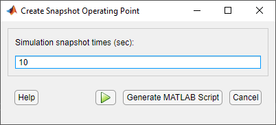
To take a snapshot of the system at the specified time, click .
The snapshot, op1, appears in the Data Browser, in the Operating Points section and contains all of the system state values at the specified time.
On the Steady State tab, click Trim Specification.
To Initialize the operating point states with the simulation snapshot values, on the Specification tab, click Initialize From , and select op1.
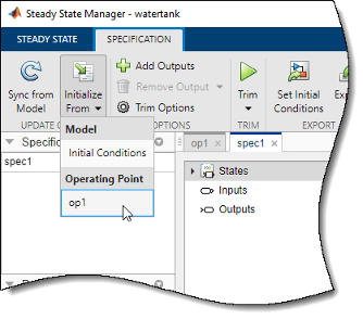
In the spec1 document, the displayed state values update to reflect the imported values.
To find the optimized operating point using the states at t = 10 as the initial values, on the Specification tab, click Trim . The software trims the model and generates an operating point search report.
In the report1 document, the Actual dx values are at or near zero, showing that the operating point is at a steady state.

Initialize Operating Point Search Using Model Linearizer

You can initialize operating point searches with a simulation snapshot when computing operating points using the Model Linearizer.

Open the Simulink model.
```
sys = ('watertank');
open_system(sys)
```
In the Simulink model window, in the Apps gallery, click Model Linearizer.
In the Model Linearizer, in the Operating Point drop-down list, click Take Simulation Snapshot.
In the Enter snapshot times to linearize dialog box, enter 10 in the Simulation snapshot times field to extract the operating point at this simulation time.
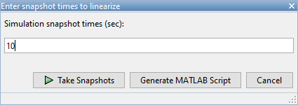
To take a snapshot of the system at the specified time, click Take Snapshots.
The snapshot, op_snapshot1, appears in the Data Browser, in the Linear Analysis Workspace section and contains all the system state values at the specified time.
On the Linear Analysis tab, in the Operating Point drop-down list, click Trim Model.
To Initialize the operating point states with the simulation snapshot values, in the Trim the model dialog box, click Import.
In the Import initial values and specifications dialog box, select op_snapshot1, and click Import.
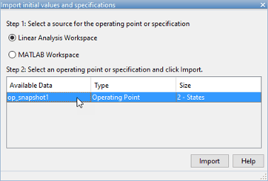
In the Trim the model dialog box, the displayed state values update to reflect the imported values.
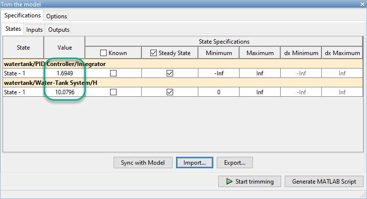
To find the optimized operating point using the states at t = 10 as the initial values, click Start trimming.
To evaluate whether the resulting operating point values meet the specifications, in the Data Browser, in the Linear Analysis Workspace section, double-click op_trim1.
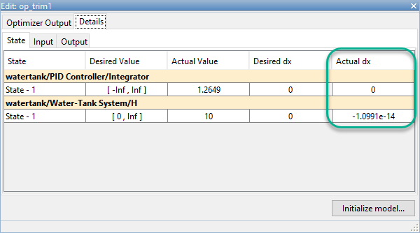
The Actual dx values are at or near zero, showing that the operating point is at a steady state.

Initialize Operating Point Search at the Command Line

Open Live Script

You can initialize operating point searches with a simulation snapshot when computing operating points using the findop function.

Open the Simulink model.

sys = 'watertank';
load_system(sys)

Simulate the model until it reaches a steady state, and extract an operating point snapshot. For this example, use ten time units.

opsim = findop(sys,10);

Create an operating point specification object. By default, all model states are specified to be at steady state.

opspec = operspec(sys);

Configure initial values for operating point search using the snapshot data.

opspec = initopspec(opspec,opsim);

Find the steady-state operating point that meets these specifications.

[op,opreport] = findop(sys,opspec);

 Operating point search report:
---------------------------------

 Operating point search report for the Model watertank.
 (Time-Varying Components Evaluated at time t=10)

Operating point specifications were successfully met.
States: 
----------
(1.) watertank/PID Controller/Integrator/Continuous/Integrator
      x:          1.26      dx:             0 (0)
(2.) watertank/Water-Tank System/H
      x:            10      dx:      -1.1e-14 (0)

Inputs: None 
----------

Outputs: None 
----------

The time derivative of each state, dx, is effectively zero. This value of the state derivative indicates that the operating point is at steady state.

Documentation