You can find a steady-state operating point using a model simulation. The resulting operating point consists of the state values and model input levels at a specified simulation snapshot time.
To use simulation-based operating point computation, first configure your model
initial conditions such that the model converges to an equilibrium point. You can
then simulate your model and create operating points interactively using the
Steady State Manager or Model Linearizer. You can also
find snapshots programmatically at the MATLAB® command line using the findop function.
To find operating points using snapshots, the software simulates the model and creates an operating point at each simulation snapshot time. Each operating point contains the input and states values of the model at the corresponding snapshot time.
To verify that the operating point is at steady state, initialize your model with the operating point values, simulate the model, and check if key signals and states are at equilibrium. For more information on initializing your model with an operating point, see Simulate Simulink Model at Specific Operating Point.
Note
If your Simulink® model contains blocks with internal states, do not linearize the model at an operating point you compute from a simulation snapshot. Instead, try linearizing the model using a simulation snapshot or at an operating point found using trimming.
You can find an operating point at specified simulation snapshot times using the Steady State Manager.
Open the Simulink model.
sys = 'magball';
open_system(sys)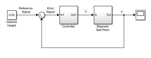
To open the Steady State Manager, in the Simulink model window, in the Apps gallery, click Steady State Manager.
To specify the simulation snapshot time, in the Steady State Manager, on the Steady State tab, click Snapshots.
Specify simulation ties at which to take snapshots. For this example, take
snapshots 1 and 10 time units. In the
Create Snapshot Operating Point dialog box, in the Simulation
snapshot times field, enter [1
10].
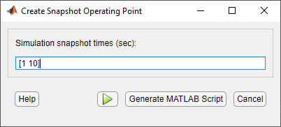
To take the snapshots, click ![]() .
.
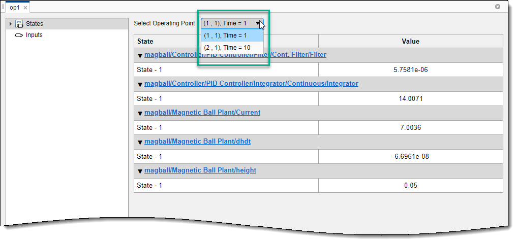
An array of operating points, op1, appears in the
Data Browser, in the Operating
Points section. This array contains two operating points,
one for each specified snapshot time.
The software also opens a corresponding op1 document where you can view the operating points.
To select which operating point to view, use the Select Operating Point drop-down list.
You can find an operating point at specified simulation snapshot times using the Model Linearizer.
Open the Simulink model.
sys = 'magball';
open_system(sys)
To open the Model Linearizer, in the Simulink model window, in the Apps gallery, click Model Linearizer.
To specify the simulation snapshot time, in the Model Linearizer,
on the Linear Analysis tab, in the Operating
Point drop-down list, select Take Simulation
Snapshot.
Take simulation snapshots at 1 and 10
time units. In the Enter snapshot times to linearize dialog box, in the
Simulation snapshot times field, enter
[1
                        10]
.
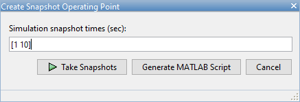
To take the snapshots, click Take Snapshots.
An array of operating points, op_snapshot1, appears in
the Data Browser, in the Linear Analysis
Workspace section. This array contains two operating
points, one for each specified snapshot time.
To view the operating points, in the Linear Analysis
Workspace, double-click op_snapshot1.
You can select which operating point to view using the Select
Operating Point drop-down list.
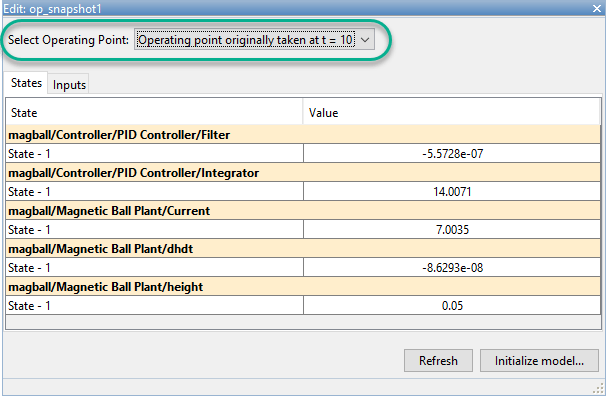
This example shows how to compute a steady-state operating point at specified simulation snapshot times.
Open the Simulink model.
sys = 'magball';
open_system(sys)

Simulate the model, and create operating points at 1 and 10 time units. The software simulates the model and computes an operating point at each simulation snapshot time.
op = findop(sys,[1 10]);
op is a column vector of operating points, with one element for each specified snapshot time.
Display the first operating point.
op(1)
 Operating point for the Model magball.
 (Time-Varying Components Evaluated at time t=1)

States:
----------
(1.) magball/Controller/PID Controller/Filter/Cont. Filter/Filter
      x: 5.76e-06
(2.) magball/Controller/PID Controller/Integrator/Continuous/Integrator
      x: 14
(3.) magball/Magnetic Ball Plant/Current
      x: 7
(4.) magball/Magnetic Ball Plant/dhdt
      x: -6.7e-08
(5.) magball/Magnetic Ball Plant/height
      x: 0.05

Inputs: None
----------