monopoleCylindrical

Create cylindrical monopole antenna over rectangular ground plane

Description

The monopoleCylindrical object is a cylindrical monopole antenna mounted over a rectangular ground plane. This antenna is useful for designing thicker monopole antennas. These antennas are mostly used in wireless mobile communication due to their broadband characteristics and simple design.

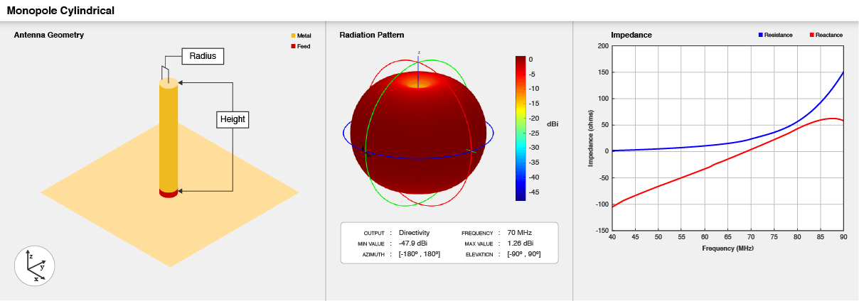
Cylindrical monopole antenna geometry, default radiation pattern, and impedance plot.

Creation

Syntax

ant = monopoleCylindrical

ant = monopoleCylindrical(Name,Value)

Description

example

ant = monopoleCylindrical creates a cylindrical monopole antenna object with default dimensions for an operating frequency of 70 MHz.

example

ant = monopoleCylindrical(Name,Value) sets Properties using one or more name-value pairs. For example, ant = monopoleCylindrical('Radius',0.04), creates a cylindrical monopole antenna with a radius of 0.04 meters.

Properties

expand all

`Height` — Height of monopole along z-axis
`1` (default) | positive scalar

Height of the monopole along the z-axis, specified as a positive scalar in meters.

Example: 'Height',3

Data Types: double

`Radius` — Radius of monopole
`0.040` (default) | positive scalar

Radius of the monopole, specified as a positive scalar in meters.

Example: 'Radius',0.05

Data Types: double

`GroundPlaneLength` — Ground plane length along x-axis
`2` (default) | positive scalar

Ground plane length along x-axis, specified as a positive scalar in meters.

Example: 'GroundPlaneLength',4

Data Types: double

`GroundPlaneWidth` — Ground plane width along y-axis
`2` (default) | positive scalar

Ground plane width along y-axis, specified as a positive scalar in meters.

Example: 'GroundPlaneWidth',2.5

Data Types: double

`FeedOffset` — Signed distance from center along length and width of ground plane
`[0 0]` (default) | two-element vector

Signed distance from the center along the length and the width of the ground plane, specified as a two-element vector in meters.

Example: 'FeedOffset',[2 1]

Data Types: double

`ClosedEnd` — Determines if monopole top is closed with cap
`0` (default) | `1`

Determine if the monopole top is closed with a cap or left open, specified as 0 or 1. Specify 1 for a closed-top monopole, and 0 for an open-top monopole.

Example: 'ClosedEnd',1

Data Types: double

`Conductor` — Type of metal material
`'PEC'` (default) | `metal` object

Type of the metal used as a conductor, specified as a metal material object. You can choose any metal from the MetalCatalog or specify a metal of your choice. For more information, see metal. For more information on metal conductor meshing, see Meshing.

Example: m = metal('Copper'); 'Conductor',m

Example: m = metal('Copper'); ant.Conductor = m

`Tilt` — Tilt angle of antenna
`0` (default) | scalar | vector

Tilt angle of the antenna, specified as a scalar or vector with each element unit in degrees. For more information, see Rotate Antennas and Arrays.

Example: 'Tilt',90

Example: ant.Tilt = 90

Example: 'Tilt',[90 90],'TiltAxis',[0 1 0;0 1 1] tilts the antenna at 90 degrees about the two axes defined by the vectors.

Data Types: double

`TiltAxis` — Tilt axis of antenna
`[1 0 0]` (default) | three-element vector of Cartesian coordinates | two three-element vectors of Cartesian coordinates | `'X'` | `'Y'` | `'Z'`

Tilt axis of the antenna, specified as:

Three-element vector of Cartesian coordinates in meters. In this case, each coordinate in the vector starts at the origin and lies along the specified points on the X-, Y-, and Z-axes.
Two points in space, each specified as three-element vectors of Cartesian coordinates. In this case, the antenna rotates around the line joining the two points in space.
A string input describing simple rotations around one of the principal axes, 'X', 'Y', or 'Z'.

For more information, see Rotate Antennas and Arrays.

Example: 'TiltAxis',[0 1 0]

Example: 'TiltAxis',[0 0 0;0 1 0]

Example: ant.TiltAxis = 'Z'

Data Types: double

`Load` — Lumped elements
[1x1 `lumpedElement`] (default) | `lumpedElement` object

Lumped elements added to the antenna feed, specified as a lumpedElement object handle. You can add a load anywhere on the surface of the antenna. By default, the load is at the feed. For more information, see lumpedElement.

Example: 'Load',lumpedelement, where lumpedelement is the load added to the antenna feed.

Example: ant.Load = lumpedElement('Impedance',75)

Object Functions

`show`	Display antenna or array structure; display shape as filled patch
`axialRatio`	Axial ratio of antenna
`beamwidth`	Beamwidth of antenna
`charge`	Charge distribution on metal or dielectric antenna or array surface
`current`	Current distribution on metal or dielectric antenna or array surface
`cylinder2strip`	Cylinder equivalent width approximation
`design`	Design prototype antenna or arrays for resonance at specified frequency
`efficiency`	Radiation efficiency of antenna
`EHfields`	Electric and magnetic fields of antennas; Embedded electric and magnetic fields of antenna element in arrays
`impedance`	Input impedance of antenna; scan impedance of array
`mesh`	Mesh properties of metal or dielectric antenna or array structure
`meshconfig`	Change mesh mode of antenna structure
`optimize`	Optimize antenna or array using SADEA optimizer
`pattern`	Radiation pattern and phase of antenna or array; Embedded pattern of antenna element in array
`patternAzimuth`	Azimuth pattern of antenna or array
`patternElevation`	Elevation pattern of antenna or array
`rcs`	Calculate and plot radar cross section (RCS) of platform, antenna, or array
`returnLoss`	Return loss of antenna; scan return loss of array
`sparameters`	S-parameter object
`strip2cylinder`	Calculates equivalent radius approximation for strip
`vswr`	Voltage standing wave ratio of antenna

Examples

collapse all

Create Default Cylindrical Monopole Antenna and Plot Radiation Pattern

Open Live Script

Create a cylindrical monopole antenna with default properties.

ant = monopoleCylindrical

ant = 
  monopoleCylindrical with properties:

               Height: 1
               Radius: 0.0400
    GroundPlaneLength: 2
     GroundPlaneWidth: 2
           FeedOffset: [0 0]
            ClosedEnd: 0
            Conductor: [1x1 metal]
                 Tilt: 0
             TiltAxis: [1 0 0]
                 Load: [1x1 lumpedElement]

View the antenna using the show function.

show(ant)

Figure contains an axes. The axes with title monopoleCylindrical antenna element contains 4 objects of type patch, surface. These objects represent PEC, feed.

Plot the radiation pattern of cylindrical monopole antenna at a frequency of 70 MHz.

pattern(ant,70e6)

Figure contains an axes and other objects of type uicontrol. The axes contains 4 objects of type patch, surface.

Plot S-Parameter of Cylindrical Monopole Antenna

Open Live Script

Create a cylindrical monopole antenna with length and radius as 1 m and 50 mm respectively.

ant = monopoleCylindrical;
ant.Height = 1;
ant.Radius = 50e-3

ant = 
  monopoleCylindrical with properties:

               Height: 1
               Radius: 0.0500
    GroundPlaneLength: 2
     GroundPlaneWidth: 2
           FeedOffset: [0 0]
            ClosedEnd: 0
            Conductor: [1x1 metal]
                 Tilt: 0
             TiltAxis: [1 0 0]
                 Load: [1x1 lumpedElement]

Visualize the antenna using show function.

show(ant)

Figure contains an axes. The axes with title monopoleCylindrical antenna element contains 4 objects of type patch, surface. These objects represent PEC, feed.

Plot the S-parameters over a frequency range of 30 MHz to 120 MHz.

s = sparameters(ant,linspace(30e6,120e6,51));
rfplot(s)

$Figure contains an axes. The axes contains an object of type line. This object represents dB(S_{11}).$

Compare Current Distribution of Open-ended and Closed-ended Cylindrical Monopole Antenna

Open Live Script

Create cylindrical monopole antennas with an open-ended top and a closed-ended top respectively.

ant = monopoleCylindrical("Radius",0.1);
ant_ClosedEnded = monopoleCylindrical("Radius",0.1,"ClosedEnd",1);

Calculate and plot the current distribution for a cylindrical monopole antennas at 70 MHz frequency.

I_OpenEnded = current(ant,70e6)

I_OpenEnded = 3×334 complex

  -0.0105 + 0.0033i  -0.0001 + 0.0000i   0.0063 - 0.0024i  -0.0008 + 0.0004i   0.0222 - 0.0056i  -0.0013 + 0.0005i  -0.0575 + 0.0053i  -0.0037 + 0.0017i   0.0013 - 0.0005i   0.0120 - 0.0039i   0.0005 - 0.0002i   0.0111 - 0.0034i   0.0083 - 0.0029i  -0.0346 + 0.0034i  -0.0021 + 0.0010i  -0.0108 + 0.0034i  -0.0129 + 0.0033i  -0.0011 + 0.0002i  -0.0007 + 0.0003i  -0.0061 + 0.0023i   0.0038 - 0.0010i  -0.0034 + 0.0011i  -0.0064 + 0.0023i  -0.0059 + 0.0022i  -0.0040 + 0.0019i  -0.0226 + 0.0061i  -0.0216 + 0.0059i  -0.0084 + 0.0029i   0.0022 - 0.0012i  -0.0383 + 0.0074i  -0.0084 + 0.0029i  -0.0034 + 0.0017i   0.0224 - 0.0061i   0.0582 - 0.0050i   0.0155 - 0.0042i  -0.0137 + 0.0044i   0.0008 + 0.0003i  -0.0140 + 0.0043i   0.0580 - 0.0052i  -0.0367 + 0.0032i   0.0008 - 0.0004i   0.0312 - 0.0062i   0.0007 - 0.0003i   0.0123 - 0.0020i   0.0032 - 0.0014i   0.0009 - 0.0005i  -0.0112 + 0.0037i  -0.0037 + 0.0017i   0.0019 - 0.0007i  -0.0002 - 0.0002i
   0.0096 - 0.0028i   0.0053 - 0.0020i   0.0030 - 0.0013i   0.0039 - 0.0019i   0.0073 - 0.0018i   0.0084 - 0.0030i   0.0207 - 0.0015i   0.0007 - 0.0003i   0.0081 - 0.0029i   0.0054 - 0.0018i   0.0247 - 0.0062i   0.0081 - 0.0025i   0.0027 - 0.0009i   0.0505 - 0.0044i   0.0034 - 0.0017i  -0.0084 + 0.0025i  -0.0189 + 0.0048i  -0.0240 + 0.0061i  -0.0037 + 0.0017i  -0.0065 + 0.0023i   0.0246 - 0.0065i   0.0085 - 0.0030i   0.0061 - 0.0023i   0.0062 - 0.0022i   0.0008 - 0.0004i  -0.0061 + 0.0017i   0.0059 - 0.0017i   0.0026 - 0.0009i  -0.0009 + 0.0005i   0.0003 + 0.0001i  -0.0027 + 0.0009i   0.0021 - 0.0010i   0.0058 - 0.0016i   0.0181 - 0.0018i  -0.0174 + 0.0047i  -0.0001 + 0.0000i   0.0620 - 0.0054i   0.0007 - 0.0002i  -0.0187 + 0.0014i  -0.0496 + 0.0046i  -0.0039 + 0.0019i  -0.0227 + 0.0040i   0.0037 - 0.0017i   0.0374 - 0.0072i   0.0039 - 0.0018i   0.0022 - 0.0011i   0.0044 - 0.0016i  -0.0007 + 0.0003i   0.0084 - 0.0029i  -0.0619 + 0.0056i
   0.0000 + 0.0000i   0.0000 + 0.0000i   0.0000 + 0.0000i   0.0000 + 0.0000i   0.0000 + 0.0000i   0.0000 + 0.0000i   0.0000 + 0.0000i   0.0000 + 0.0000i   0.0000 + 0.0000i   0.0000 + 0.0000i   0.0000 + 0.0000i   0.0000 + 0.0000i   0.0000 + 0.0000i   0.0000 + 0.0000i   0.0000 + 0.0000i   0.0000 + 0.0000i   0.0000 + 0.0000i   0.0000 + 0.0000i   0.0000 + 0.0000i   0.0000 + 0.0000i   0.0000 + 0.0000i   0.0000 + 0.0000i   0.0000 + 0.0000i   0.0000 + 0.0000i   0.0000 + 0.0000i   0.0000 + 0.0000i   0.0000 + 0.0000i   0.0000 + 0.0000i   0.0000 + 0.0000i   0.0000 + 0.0000i   0.0000 + 0.0000i   0.0000 + 0.0000i   0.0000 + 0.0000i   0.0000 + 0.0000i   0.0000 + 0.0000i   0.0000 + 0.0000i   0.0000 + 0.0000i   0.0000 + 0.0000i   0.0000 + 0.0000i   0.0000 + 0.0000i   0.0000 + 0.0000i   0.0000 + 0.0000i   0.0000 + 0.0000i   0.0000 + 0.0000i   0.0000 + 0.0000i   0.0000 + 0.0000i   0.0000 + 0.0000i   0.0000 + 0.0000i   0.0000 + 0.0000i   0.0000 + 0.0000i

current(ant,70e6)

Figure contains an axes. The axes with title Current distribution contains 4 objects of type patch.

I_ClosedEnded = current(ant_ClosedEnded,70e6)

I_ClosedEnded = 3×342 complex

  -0.0095 + 0.0039i  -0.0001 + 0.0000i   0.0057 - 0.0027i  -0.0007 + 0.0004i   0.0201 - 0.0069i  -0.0012 + 0.0006i  -0.0522 + 0.0084i  -0.0034 + 0.0019i   0.0012 - 0.0006i   0.0109 - 0.0045i   0.0005 - 0.0003i   0.0101 - 0.0041i   0.0076 - 0.0034i  -0.0314 + 0.0053i  -0.0019 + 0.0011i  -0.0098 + 0.0040i  -0.0117 + 0.0041i  -0.0010 + 0.0003i  -0.0006 + 0.0003i  -0.0056 + 0.0026i   0.0035 - 0.0012i  -0.0031 + 0.0013i  -0.0059 + 0.0026i  -0.0054 + 0.0025i  -0.0036 + 0.0021i  -0.0206 + 0.0074i  -0.0197 + 0.0071i  -0.0076 + 0.0034i   0.0020 - 0.0013i  -0.0348 + 0.0095i  -0.0076 + 0.0034i  -0.0031 + 0.0019i   0.0204 - 0.0073i   0.0528 - 0.0082i   0.0141 - 0.0050i  -0.0125 + 0.0052i   0.0007 + 0.0003i  -0.0127 + 0.0050i   0.0526 - 0.0084i  -0.0333 + 0.0052i   0.0007 - 0.0004i   0.0283 - 0.0079i   0.0006 - 0.0003i   0.0112 - 0.0027i   0.0029 - 0.0016i   0.0008 - 0.0005i  -0.0102 + 0.0043i  -0.0034 + 0.0019i   0.0018 - 0.0008i  -0.0002 - 0.0002i
   0.0087 - 0.0034i   0.0048 - 0.0023i   0.0028 - 0.0014i   0.0036 - 0.0021i   0.0067 - 0.0022i   0.0076 - 0.0035i   0.0188 - 0.0026i   0.0006 - 0.0003i   0.0073 - 0.0034i   0.0049 - 0.0021i   0.0225 - 0.0075i   0.0074 - 0.0029i   0.0024 - 0.0011i   0.0458 - 0.0071i   0.0031 - 0.0019i  -0.0077 + 0.0030i  -0.0171 + 0.0058i  -0.0218 + 0.0074i  -0.0034 + 0.0019i  -0.0059 + 0.0027i   0.0224 - 0.0079i   0.0078 - 0.0034i   0.0056 - 0.0026i   0.0056 - 0.0025i   0.0007 - 0.0004i  -0.0055 + 0.0020i   0.0054 - 0.0020i   0.0023 - 0.0010i  -0.0008 + 0.0005i   0.0003 + 0.0001i  -0.0024 + 0.0011i   0.0019 - 0.0011i   0.0053 - 0.0019i   0.0164 - 0.0027i  -0.0158 + 0.0057i  -0.0001 + 0.0000i   0.0563 - 0.0089i   0.0006 - 0.0002i  -0.0170 + 0.0024i  -0.0450 + 0.0074i  -0.0036 + 0.0021i  -0.0206 + 0.0053i   0.0033 - 0.0019i   0.0340 - 0.0092i   0.0035 - 0.0021i   0.0020 - 0.0013i   0.0040 - 0.0018i  -0.0006 + 0.0003i   0.0077 - 0.0034i  -0.0562 + 0.0090i
   0.0000 + 0.0000i   0.0000 + 0.0000i   0.0000 + 0.0000i   0.0000 + 0.0000i   0.0000 + 0.0000i   0.0000 + 0.0000i   0.0000 + 0.0000i   0.0000 + 0.0000i   0.0000 + 0.0000i   0.0000 + 0.0000i   0.0000 + 0.0000i   0.0000 + 0.0000i   0.0000 + 0.0000i   0.0000 + 0.0000i   0.0000 + 0.0000i   0.0000 + 0.0000i   0.0000 + 0.0000i   0.0000 + 0.0000i   0.0000 + 0.0000i   0.0000 + 0.0000i   0.0000 + 0.0000i   0.0000 + 0.0000i   0.0000 + 0.0000i   0.0000 + 0.0000i   0.0000 + 0.0000i   0.0000 + 0.0000i   0.0000 + 0.0000i   0.0000 + 0.0000i   0.0000 + 0.0000i   0.0000 + 0.0000i   0.0000 + 0.0000i   0.0000 + 0.0000i   0.0000 + 0.0000i   0.0000 + 0.0000i   0.0000 + 0.0000i   0.0000 + 0.0000i   0.0000 + 0.0000i   0.0000 + 0.0000i   0.0000 + 0.0000i   0.0000 + 0.0000i   0.0000 + 0.0000i   0.0000 + 0.0000i   0.0000 + 0.0000i   0.0000 + 0.0000i   0.0000 + 0.0000i   0.0000 + 0.0000i   0.0000 + 0.0000i   0.0000 + 0.0000i   0.0000 + 0.0000i   0.0000 + 0.0000i

figure;
current(ant_ClosedEnded,70e6)

Figure contains an axes. The axes with title Current distribution contains 4 objects of type patch.

More About

expand all

Parametric Analysis Guidelines

To understand how the properties of the monopoleCylindrical antenna object influence the antenna design, use the following parametric analysis guidelines.

To increase the operating frequency, decrease the Height of the monopoleCylindrical antenna.
To increase the gain, increase the ground plane dimensions of the monopoleCylindrical antenna object using the GroundPlaneLength and the GroundPlaneWidth properties.
To increase the bandwidth, increase the radius and change the feed location of the monopoleCylindrical antenna object using the Radius and the FeedOffset properties.

References

[1] King, Ronald W.P. Characteristics of Cylindrical Dipoles and Monopoles. Boston, MA: Springer, 1971.

Documentation

monopoleCylindrical

Description

Creation

Syntax

Description

Properties

`Height` — Height of monopole along z-axis
`1` (default) | positive scalar

`Radius` — Radius of monopole
`0.040` (default) | positive scalar

`GroundPlaneLength` — Ground plane length along x-axis
`2` (default) | positive scalar

`GroundPlaneWidth` — Ground plane width along y-axis
`2` (default) | positive scalar

`FeedOffset` — Signed distance from center along length and width of ground plane
`[0 0]` (default) | two-element vector

`ClosedEnd` — Determines if monopole top is closed with cap
`0` (default) | `1`

`Conductor` — Type of metal material
`'PEC'` (default) | `metal` object

`Tilt` — Tilt angle of antenna
`0` (default) | scalar | vector

`TiltAxis` — Tilt axis of antenna
`[1 0 0]` (default) | three-element vector of Cartesian coordinates | two three-element vectors of Cartesian coordinates | `'X'` | `'Y'` | `'Z'`

`Load` — Lumped elements
[1x1 `lumpedElement`] (default) | `lumpedElement` object

Object Functions

Examples

Create Default Cylindrical Monopole Antenna and Plot Radiation Pattern

Plot S-Parameter of Cylindrical Monopole Antenna

Compare Current Distribution of Open-ended and Closed-ended Cylindrical Monopole Antenna

More About

Parametric Analysis Guidelines

References

See Also

Topics

Antenna Toolbox Documentation

Support

Documentation

monopoleCylindrical

Description

Creation

Syntax

Description

Properties

Height — Height of monopole along z-axis 1 (default) | positive scalar

Radius — Radius of monopole 0.040 (default) | positive scalar

GroundPlaneLength — Ground plane length along x-axis 2 (default) | positive scalar

GroundPlaneWidth — Ground plane width along y-axis 2 (default) | positive scalar

FeedOffset — Signed distance from center along length and width of ground plane [0 0] (default) | two-element vector

ClosedEnd — Determines if monopole top is closed with cap 0 (default) | 1

Conductor — Type of metal material 'PEC' (default) | metal object

Tilt — Tilt angle of antenna 0 (default) | scalar | vector

TiltAxis — Tilt axis of antenna [1 0 0] (default) | three-element vector of Cartesian coordinates | two three-element vectors of Cartesian coordinates | 'X' | 'Y' | 'Z'

Load — Lumped elements [1x1 lumpedElement] (default) | lumpedElement object

Object Functions

Examples

Create Default Cylindrical Monopole Antenna and Plot Radiation Pattern

Plot S-Parameter of Cylindrical Monopole Antenna

Compare Current Distribution of Open-ended and Closed-ended Cylindrical Monopole Antenna

More About

Parametric Analysis Guidelines

References

See Also

Topics

Antenna Toolbox Documentation

Support

`Height` — Height of monopole along z-axis
`1` (default) | positive scalar

`Radius` — Radius of monopole
`0.040` (default) | positive scalar

`GroundPlaneLength` — Ground plane length along x-axis
`2` (default) | positive scalar

`GroundPlaneWidth` — Ground plane width along y-axis
`2` (default) | positive scalar

`FeedOffset` — Signed distance from center along length and width of ground plane
`[0 0]` (default) | two-element vector

`ClosedEnd` — Determines if monopole top is closed with cap
`0` (default) | `1`

`Conductor` — Type of metal material
`'PEC'` (default) | `metal` object

`Tilt` — Tilt angle of antenna
`0` (default) | scalar | vector

`TiltAxis` — Tilt axis of antenna
`[1 0 0]` (default) | three-element vector of Cartesian coordinates | two three-element vectors of Cartesian coordinates | `'X'` | `'Y'` | `'Z'`

`Load` — Lumped elements
[1x1 `lumpedElement`] (default) | `lumpedElement` object